Don't Fear the Smith Chart
- Dan Koellen AI6XG
- Jun 15, 2021
- 13 min read
Updated: Jun 18, 2021
Like many radio amateurs I was initially intimidated by the Smith chart. Transmission line and antenna theory, unfamiliar terms and concepts, and endless formulas made understanding a Smith Chart daunting. For me, after finding the right project and software, I took a less arduous path to using the Smith Chart. So join me in discovering the delight of using Smith charts.
This article will get you started on using the Smith chart. I am not, by any means, a Smith chart expert but, by showing how to design a LC matching network, I will whet your appetite to learn more about Smith charts. Some math will be necessary but should not overwhelm you. Likewise, understanding of a couple basic transmission and antenna terms will be required. Just a general understanding of the concepts will suffice for now, software will allow us to build the matching network using a Smith chart without having to perform the calculations ourselves. And you will see the effect of each network component on the Smith chart. This will make it easier to go back and understand the theory and math behind the Smith chart should you choose to.
What is a Smith chart?
The Smith chart, invented by Phillip H. Smith, has been described in complex terms such as being a graphical calculator plotted on a complex coefficient reflection plane or a Moebius transform from complex impedance plane to the Gamma plane among other obfuscating, though technically correct, descriptions.
In simple terms, a Smith chart is a map from one impedance to another impedance. In most cases an antenna, filter or amplifier is a load that needs its impedance, noted as ZL, mapped (matched) to a system impedance, noted as Z0. The impedance Z0 is 50 ohms in most cases, quite often the output of your rig. Each component in the matching network between the impedances are represented on the Smith chart by a circular path. The Smith chart helps you find the right component and connection to find your way along these circular paths from ZL to Z0.
Though the Smith chart started out as a paper chart, software programs are now used. A free program written by AE6TY is SimSmith. Go ahead and download the program to follow along with the examples that I will go through here. The download page also has links to introductory videos and tutorials. SimSmith is a very useful program that makes using a Smith chart a snap.
A Review of a Few Basics
To follow along our Smith chart journey I will remind you of a few basic items that we learned to pass our amateur radio licence exams. Take a look and you can always reference back if you need to when we design the matching networks.
All impedances are a complex number, meaning it has a real component and an imaginary component. The real part, R, is resistance and the imaginary part, jX, is reactance (X) which is associated with either a capacitor or inductor multiplied by j (where j is the square root of -1). Don't worry about j, the important thing to remember is the role of resistance and reactance.
Z = R + jX where X < 0 for capacitors X > 0 for inductors
Also remember that impedances and resistances in series add:
Zs = Z1 + Z2 and Rs = R1 + R2
Impedance and resistance in parallel do not add but their reciprocals do add in parallel. Conductance (G) is the reciprocal of resistance and admittance (Y) is the reciprocal of impedance. Since impedance is a complex number the reciprocal is also a complex number. For now, remember what G and Y stand for:
G = 1/R Y = 1/Z
and that they add in parallel:
G|| = G1 + G2 and Y|| = Y1 + Y2
One transmission term is needed, that is the Reflection Coefficient. Normally the reflection coefficient is represented by a capital Gamma but I will use T since I am limited in fonts that are available in this blog. The reflection coefficient is simply the ratio of the reflected wave and incident wave in a transmission line. The are several relationships that may be derived involving the reflection coefficient but only one is important at this point:
T = (ZL - Z0)/(ZL + Z0)
Since impedances are complex numbers the reflection coefficient is also a complex number. Here ZL and Z0 are the load and system impedances we discussed earlier, making T an interesting relationship. Math operations on complex numbers can be tricky but software will take care of it for you.
Smith Chart Basics
An interesting property of the reflection coefficient is that is bounded by -1 and 1 for any value of ZL, this is a circle of radius 1 giving the Smith chart its shape. So any value of ZL may be plotted on the Smith chart where the imaginary portion of T is plotted on the y axis and the real portion of T plotted on the x axis. The center of the chart, T = 0 + j0, is Z0 = ZL, T = 1 + j0 when ZL approaches infinity (open) and T = -1 + j0 when ZL = 0 (short). The top half of the Smith chart is positive reactance so it is inductive and the bottom half is negative reactance so it is capacitive.
There are a few interesting characteristics of the Smith chart that come in handy when designing matching networks. On the chart, the graph of constant resistance (real part) with all values of reactance (imaginary part representing a capacitor of inductor) is a circle.


Plots of Constant Resistance L to R 125 Ohms, 50 Ohms, 12.5 Ohms
Likewise, the plot of constant conductance with all values of reactance (imaginary part representing a capacitor of inductor) is a circle..


Plots of Constant Conductance L to R 0.05 S, 0.02 S, 0.008 S
In these plots, the value of T moves along this circle as the value of the reactance changes, i.e. as the value of a capacitor or inductor changes. Two important plots are the 50 Ohm and 0.02 S circles that go through the center of the graph where ZL = Z0. This is the desired endpoint for a matching network.
Using a Smith Chart to Build a Simple Matching Network
We now know enough to build a two element LC network to match a load impedance ZL to the system impedance Z0. Using the constant resistance and conductance curves we will transform the ZL to Z0.
Always starting at the point on the Smith chart for ZL (i.e. T = (ZL -Z0)/(ZL + Z0)) we will use a reactance to move to either the 50 Ohm or 0.02 S curve, then the opposite reactance to move along that curve to the center of the chart where ZL = Z0. But how will we know whether to use an inductor or capacitor in parallel or series? This is already determined; I will use some figures from Phillip Smith's 1969 landmark book 'Electronic Applications of the Smith Chart' to show typical networks.

In the chart above, ZL is in the upper half of the Smith chart so it is inductive. Starting at ZL, a series capacitor will be the first path to Z0 as indicated by the LC network schematic in the figure. The path will be along a constant resistance curve since the capacitor is in series and we assume negligent resistance associated with the capacitor. The value of the capacitor will be varied (red arrow) until the reactance moves T to the constant conductance 0.02 S curve at point Z1. Then the value of the shunt inductor will be varied (blue arrow) along the 0.02S constant conductance curve until we reach the center of the graph.

In the above chart, ZL is still inductive but in a different quadrant of the chart. In this case, starting again at ZL, a shunt capacitor will be the first path to Z0 as indicated by the LC network schematic in the figure. The path will be along a constant conductance curve since the capacitor is in parallel with ZL. The value of the capacitor will be varied (red arrow) until the reactance moves T to the constant resistance 50 Ohm curve at point Z1. Then the value of the series inductor will be varied (blue arrow) until we reach the center of the graph.
Similar paths are used for ZL that fall in the other quadrants of the Smith chart as shown below. As above, the inductor action is the blue arrow and capacitor action is the red arrow. Remember, always start at ZL.


Let's Build a LC Matching Network
I will show a couple examples of networks I have built using the Smith chart to determine the configuration and component values. Instead of using a paper chart I use SimSmith software to design the network. I will cheat a bit as well by using a web calculator by Analog Devices to get starting values for the network and use SimSmith to build a practical network using standard component values. I will assume that you have downloaded SimSmith and viewed some of the videos and tutorials on the download page.
Example 1
After building a 17 meter QCX mini, I wanted to see if I could match my trapped 20/30/40 EFHW to the QCX mini on the 17 meter band. On a SOTA summit I typically use my mtr3b with the trapped EFHW, using a 6 foot RG316 coax cable between the rig and the EFHW transformer. I decided to build a match network that would be connected between the QCX mini and the RG316 coax. Ideally I wanted to be able to swap the QCX mini and the matching network in place of the mtr3b to use 17 meters.
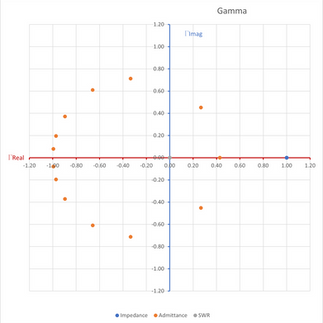
The first step was to set up the EFHW and RG316 cable and measure the impedance across the 17 meter band using the nanoVNA. The .s1p file was saved for use in SimSmith. The impedance at 18.090 MHz was determined to be 79.5 + j228.4, very inductive as expected. This is our ZL. The .s1p file is loaded into the load Z in SimSmith, try it out yourself and you should get the chart below.

To transform this impedance to 50 Ohms we will use a LC network with a shunt capacitor across ZL and a series inductor to Z0. This is a network that we saw above. Another network, with a shunt inductor across ZL and a series capacitor to Z0 could also be used. I decided not to use this network because ZL is very close to the forbidden zone for this network. Also, the network I used is a low pass filter which will give additional filtering for the rig's output.
The next step is to calculate values for the network components using an online calculator. The values will be non standard values, we will use closest standard values in SimSmith to simulate the match. Then we will use SimSmith to determine how the match changes with component values. This will determine starting values for the inductor and capacitor on the actual build as we tune it for best match.
The values we get from the online calculator are 78.643 pF and 1.629 uH. We will start with 78 pF and 1.6 uH and see how well the network matches the impedances. Of course you may just guess at a value for the first component and then adjust the value until the line meets the 50 Ohm or 0.02 S curves.
As always we start at ZL by adding a shunt 78 pF capacitor in SimSmith, we can see below that the capacitor takes the point on the chart along a constant conductance curve (green line) to the 50 Ohm constant resistance curve.

Now let's add the series 1.6 uH inductor to take the point along the 50 Ohm constant resistance curve towards the center of the chart where Z0 = ZL. The inductor is the magenta line in the chart below.

We don't quite get to the center of the chart because of a couple reasons. First we used a standard value for the inductor rather than the calculated value. Also you can see that the inductor track deviates from the constant resistance curve, this is because SimSmith models the inductor as imperfect with some series resistance. In spite of this, the match is very good with a 1.1 SWR at 18.090 MHz. Below is the SWR plot across the 17 meter band that shows a simulated SWR of less than 1.2 across the band.

Now the challenge is to build this network and see how close we can come to the simulation.
Initially I looked at how the match varies with changes in the component values. The most sensitive value seemed to be the capacitor. Changes in the capacitor value keeps the network from moving along the 50 ohm constant resistance curve to the center. Large changes in capacitor value will prevent the match to be close to the chart center, no matter the value of the inductor. This made me decide to use a set of parallel capacitors so I could fine tune the value that will provide a close match, this turned out to be a good decision. I also measured the capacitance of the BNC connector using the nanoVNA and verifying with an autozeroing small capacitance meter. The mounted BNC showed around 7 pF capacitance, leaving about 71 pF of additional capacitance. I mounted a 47 pF NP0 ceramic SMT capacitor in the BNC connector itself, followed by a 15 pF and 10 pF parallel NP0 SMT capacitors on the protoboard that the matching network was built on. This is a total of 79 pF. If needed, I could remove the 10 pF and substitute a 5 pF or 15 pF capacitor to fine tune the match.

This left the 1.6 uH inductor. I settled on 19 turns on a T50-6 toroid for the inductor using http://www.toroids.info to estimate the number of turns needed. This is just an estimate of turns since squeezing and spreading will change the inductance.

After mounting the inductor and capacitors the matching network will have to be tuned for the best match. To do this I set up the antenna and connected the matching network to the antenna through 6' of RG316 coax. The input of the matching network was fed by the nanoVNA and the Smith chart was monitored over the 17 mtr band while connected to the antenna. First I verified that the capacitance was the right value by varying the inductor and checking that the plot was traveling along a curve that will come close to the center of the chart. Then I changed the inductance by squeezing and spreading the turns until a reasonable match is made. You may find that the turns are either fully spread or squeezed which means you need to remove or add a turn respectively to the inductor. This can take some time and practice but eventually you will get a decent match. All made easier because of the Smith chart showing you the effect of changing the value of the components.


As built measurements, after potting, above show the match was very good and close to the simulation. The dashed line/circle is 1.3 SWR.
Example 2
As well as the matching network in example 1 provided a low SWR match to the rig it did not seem to be a very good antenna. Since I directly connected the matching network to my rig and then fed the output to the antenna input through 6 feet of RG316, I believe the coax was doing most of the radiating with little radiation past the EFHW transformer. So I decided to move the matching network so its output was connected directly to the EFHW transformer, that is the input of the antenna.
As in example 1, the nanoVNA was used to measure the impedance at the input of the EFHW. The .s1p file was loaded into SimSmith showing 3.381 + j15.29 impedance. The Smith chart shown below indicates that the SWR is approximately the same as the impedance in example 1 even though the impedance is different. This is to be expected since the difference in measurements was the 6' RG316 coax.

From the earlier discussion a network, starting from ZL as always, would be a series capacitor followed by a shunt inductor across the output. Using the online calculator, component values of 314 pF and 120 nH were obtained. I decided to start with standard value of 300 pF for the capacitor since I had a 200 pF and 100 pF silver mica capacitors on hand. For this version of the matching network I decided to use a male BNC at the load end and the female BNC used previously on the other end. I decided to add the capacitance of the BNC female connector to SimSmith model. I also made an estimate of the series inductance of the male BNC of 10 nH to put into the SimSmith model. In addition I added the 6' RG316 coax between the network and the rig. This is all very easy to do in SimSmith as you can see below.

Starting from the left the circuit elements are L = load, L2 = male BNC inductance, C1 = series match capacitor, L1 = shunt match inductor, C2 = female BNC capacitance, T2 = 6' RG316
As you can see most of the path to the center of the chart is due to C1 and L1. For L1 I decided to use a T37-6 toroid since changing the number of turns on a smaller toroid gives finer tuning ability. I started out with 6 turns but ended up with five widely spaced turns for a good match. In the end about 110 nH inductance was used for the match.
This version of the matching network did not achieve as low SWR as example 1 but its performance is still very good. Over the 17 meter band the SWR is less than 1.3 as shown below where the blue trace is before potting and the red trace is after potting.


The dotted line is 1.3 SWR in both charts.
The performance of this matching network and the EFHW (20, 30, 40 meter trapped) is good and preferred over example 1 configuration. My second contact using this configuration on 17 meters with 4 watts was a summit to summit contact from W6/NS-306 to W7Y/EW-017!

The simulated results and measured results (pre potting) agree very well with a shunt inductance of ~113 nH and the male BNC parasitic self inductance of 15 nH.

Lessons Learned
Here are a few things that I learned while building the matching networks that will help you with your design implementation.
When measuring ZL impedance use the nanoVNA by itself and use its file saving capability to retain the .s1p files. Some of my initial measurements where performed with the nanoVNA connected to a computer using nanoSaver software. There was just too much RFI from the laptop and power supply that was being picked up by the antenna. The readings were affected; not accurate and consistent.
The nanoVNA measured high reactance impedances better than standard antenna analyzers designed mainly for SWR measurements.
Premeasure the inductors and capacitors with the nanoVNA at the frequency of interest before using in the matching network. There are various discussions on accuracy but it will get you in the right ball park. The calculated inductance for toroids is not always close to actual value due to winding spacing and toroid material variance.
Often you have to decide whether to use n turns or n + 1 turns on a toroid. Rather than adding or subtracting turns on one toroid I wind two toroids with different number of turns. This makes it easier to play with spacing to get a targeted inductance. And I find it easier to swap out toroids than to try to remove or add turns while the toroid is mounted on the board.
I pot the assembled and tuned matching network with Gorilla Glue 5 Minute two part clear epoxy. Be sure to use clear epoxy, definitely don't use anything with metal fillers. There will be some change in characteristics after potting but nothing significant. I find that the potting is worth it to protect the board and components and keeping the toroid windings in place.
Conclusions
Smith chart software, such as SimSmith, has made using a Smith chart much easier to use and understand. Smith charts are used for much more than the above simple LC network example. I hope this has given you the motivation to further explore the Smith chart and its additional applications in more depth. Below are references that will get you further down the Smith chart path.
References
.s1p and .ssx files available here
excel spreadsheet used to produce constant R and G circles available here
YouTube
The Complete Forbidden Area Chart
